Lupine
Publishers- Biostatistics and Biometrics Open Access Journal
he four-parameter generalized lambda distribution (GLD) was proposed in [1]. We say the GLD is of type V, if the quantile function corresponds to Case(v) in of [2], that is,
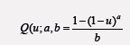 where u 2 (0, 1) and a, b 2 (−1, 0). In this short note, we introduce
the T-R {Generalized Lambda V} Families of Distributions and
show a sub-model of this class of distributions is significant in
modeling real life data, in particular the Wheaton river data, [2]. We
conjecture the new class of distributions can be used to fit biological
and health data.
where u 2 (0, 1) and a, b 2 (−1, 0). In this short note, we introduce
the T-R {Generalized Lambda V} Families of Distributions and
show a sub-model of this class of distributions is significant in
modeling real life data, in particular the Wheaton river data, [2]. We
conjecture the new class of distributions can be used to fit biological
and health data.Keywords and Phrases: Generalized Lambda Distribution; Exponential Distribution; Weibull Distribution
Contents
b) The New Distribution
c) Practical Significance
d) Open Problem
The T – R {Y} Family of Distributions
This family of distributions was proposed in [3]. In particular, let T, R, Y be random variables with CDF’s FT (x) = P (T _ x), FR(x) = P (R _ x), and FY (x) = P (Y _ x), respectively. Let the corresponding quantile functions be denoted by QT (p), QR(p), and QY (p), respectively. Also, if the densities exist, let the corresponding PDF’s be denoted by fT (x), fR(x), and fY (x), respectively. Following this notation, the, the CDF of the T – R {Y} is given by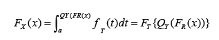 and the PDF of the T-R{Y} family is given by
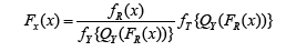
The New Distribution
Theorem: The CDF of the T-R {Generalized Lambda V} Families of Distributions is given by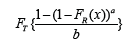 where the random variable R has CDF FR(x), the random
variable T with support (0,1) has CDF FT, and a, b 2 (−1, 0) Proof.
Consider the integral
where the random variable R has CDF FR(x), the random
variable T with support (0,1) has CDF FT, and a, b 2 (−1, 0) Proof.
Consider the integral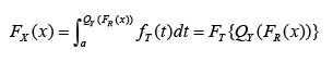 and let Y follow the generalized lambda class of distributions of
type V, where the quantile is as stated in the abstract
and let Y follow the generalized lambda class of distributions of
type V, where the quantile is as stated in the abstractRemark: the PDF can be obtained by differentiating the CDF
Practical Significance
In this section, we show a sub-model of the new distribution defined in the previous section is significant in modeling real life data. We assume T is standard exponential so that FT (t) = 1 − e−t, t > 0 and R follows the two-parameter Weibull distribution, so that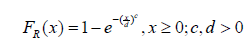 Now from Theorem 2.1, we have the following
Theorem: The CDF of the Standard Exponential-Weibull {Generalized Lambda V}
Families of Distributions is given by
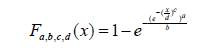 where c, d > 0 and a, b 2 (−1, 0)
By differentiating the CDF, we obtain the following
Theorem: the PDF of the Standard Exponential-Weibull {Generalized Lambda V} Families of Distributions is given by
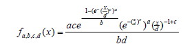 where c, d > 0 and a, b 2 (−1, 0)
Remark: If a random variable B follows the Standard Exponential-Weibull {Generalized
Lambda V} Families of Distributions write
B _ SEWGLV (a, b, c, d)
Open Problem
Conjecture: The new class of distributions can be used in forecasting and modelingn of biological and health data. Related to the above conjecture is the followingQuestion: Is there a sub-model of the T-R {Generalized Lambda V} Families of Distributions that can fit? [3] (Appendix 1) and (Figures 1-3).
Appendix 1:
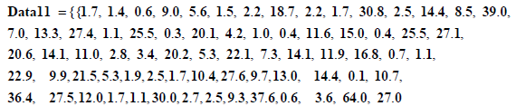 DataQ1 = Flatten Data11; Length DataQ1 72
Min DataQ1 0.1; Max DataQ1 64.
AX1 = Empirical Distribution DataQ1
Data Distribution «Empirical», { 58}
K1 = Discrete Plot [CDF [AX1, x ], {x, 0, 65, (65-0)/58} , Plot Style c {Black, Thick} , Plot Markers c {Automatic, Small} , Filling c None,
Plot Range c All]
(Figure 1)
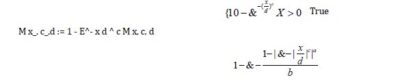
F1 x_, a_, b: = 1 - 1 - x ^ ab
CDF Weibull Distribution c, d, x
I. Weibull. nb
D 1 - E^ - F1 M x, c, d, a, b, x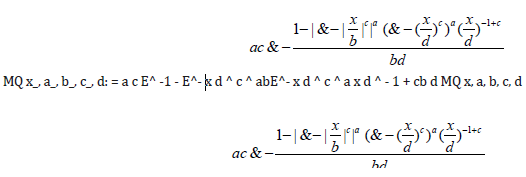 PLK1 = Sum Log MQ DataQ1, a, b, c, di, i,1, Length DataQ1;
JK=D [PLK, a];
JK1=D [PLK, b];
JK2=D [PLK, c];
JK3=D [PLK,d];
Find Root JK, JK1, JK2, JK3, a, - 0.11 ,b, - 0.12 , c, 0.9 , d, 11.6
a c – 7.2577, b c – 0.395297, c c 0.776499, d c 657.998
RR = Plot 1 - E^ - F1 M x, 0.776499, 657. 998, - 7.2577, - 0.395297, x, 0, 65, Plot Style c Thick, Blue, Plot Range c All
(Figure 2)
II. Weibull. nb
CMU = Show K1, RR, Plot Range c All
(Figure 3)
Export “CMU.jpg”, CMU CMU.jpg
Figure 1:

Figure 2:

Figure 3:

For
more Lupine Publishers Open
Access Journals Please visit our website: https://lupinepublishersgroup.com/
For
more Bio
statistics and Bio metrics Open Access Journal articles Please Click
Here: https://lupinepublishers.com/biostatistics-biometrics-journal/
To
Know More About Open
Access Publishers Please Click on Lupine
Publishers


